9 Adding non-linear effects
The previous model used only parameters. The variance explained by that model was rather small. We want to take into account the non-linear changes of f0 over time. To do that, we want to smooth these trajectories ignoring local and small changes (small amplitude wrinkles). But, we need to be careful not to over-smooth them, or we risk losing structural changes we want to keep (we want to see the rises and falls that are common for a given tone, for example).
model_02_noAR <- bam(F0_st ~
    Tone + Gender +
    s(time_norm, by = Tone, k = 10, bs = "cr") +
    s(time_norm, by = Gender, k = 10, bs = "cr") +
    s(time_norm, Speaker, bs = "fs", k = 10, m = 1) +
    s(time_norm, token, bs = "fs", k = 5, m = 1),
    data = f0_df,
    method = "fREML",
    discrete = TRUE
)
## Warning in gam.side(sm, X, tol = .Machine$double.eps^0.5): model has repeated
## 1-d smooths of same variable.model_02_noAR explains f0 trajectories over time. Tone and Gender estimate the overall f0 differences, as before. Note that there is a warning about “repeated smooths” in the model. This is caused by both Tone and Gender being modeled over the same time_norm variable and it is safe to ignore.
9.1 Factor-specific smooths
The s(time_norm, by = Tone, k = 10, bs = "cr") term allows the shape of f0 over (normalized) time to differ by Tone, so each tone receives its own “smooth” curve. k = 10 sets the maximum “wiggliness” (number of basis functions) available to each curve, and bs = "cr" picks the type of spline (cubic regression spline, a common efficient default for 1D smooths).
Figure 9.1 shows the model predicted trajectories for tones 2 and 4 together with the weighted splines used in the prediction. Any given point in the predicted trajectory (in black) is the weighted sum of the cubic regression splines at the same location. Note that even though we specified k=10, there are only 9 curves. This is due to an internal constraint in the construction of the model, so we will get k - 1 curves.
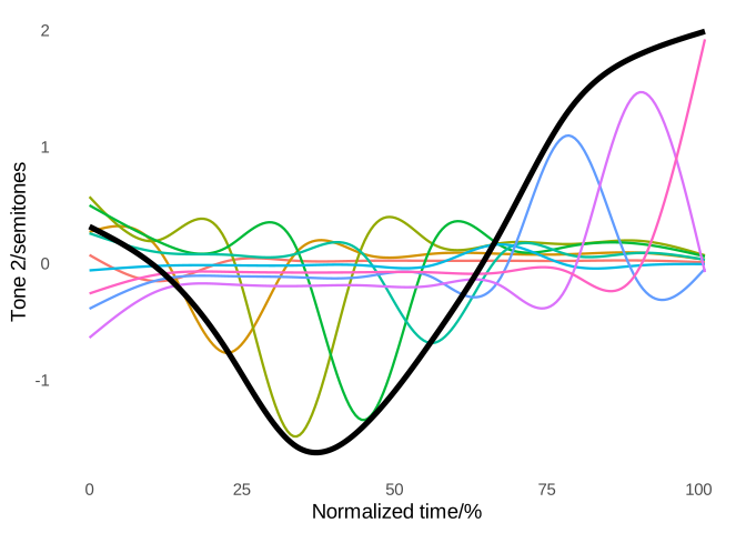
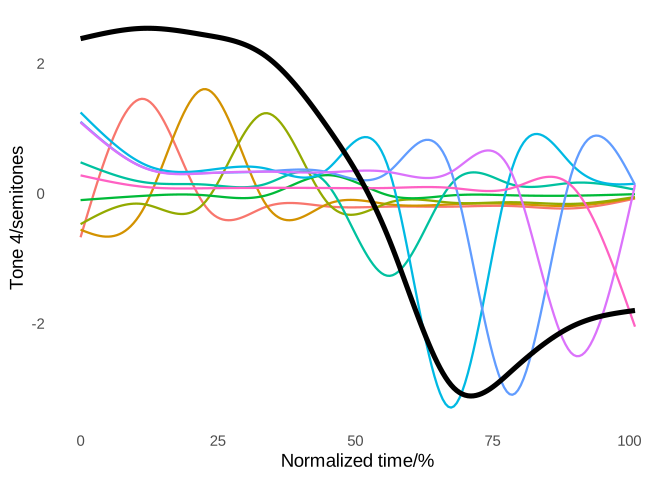
Figure 9.1: Predited tone trajectories (in black) and basis functions for Tones 2 and 4
s(time_norm, by = Gender, k = 10, bs = "cr") term does something similar for the Gender factor.
9.2 Factor smooths
The s(time_norm, Speaker, bs = "fs", k = 10, m = 1) term captures speaker-specific trajectories, i.e., it fits separate smooth trajectories for each level of speaker allowing for deviations associated with a given speaker (idiosyncrasies) from the other model terms. This would be the equivalent of a random effect in linear models. Note that we use m=1. This parameter specifies the order of the derivative used in the smoothness penalty. For the Gender and Tone smooths, we used cubic regression splines with m=2 by default. For random effects, m=1 is often preferred, instead.
- m = 1 penalizes changes in the first derivative (slope).
- m = 2 penalizes changes in the second derivative (wiggliness).
We can visualize these speaker-specific trajectories:
draw(
  model_02_noAR,
  select = "s(time_norm,Speaker)",
  rug = FALSE
) +
  theme_minimal(base_size = 14) +
  labs(
    title = NULL,
    caption = NULL,
    x = "Normalized time (%)",
    y = "F0 / semitones"
  ) +
  scale_x_continuous(
    labels = function(x) paste0(x, "%")
  ) +
  coord_cartesian(
    xlim = c(0, 100)
  ) +
  guides(
    colour = guide_legend(
      nrow = 2,
      byrow = TRUE
    )
  ) +
  theme(
    panel.grid.minor = element_blank(),
    axis.ticks = element_blank(),
    legend.position = "bottom"
) 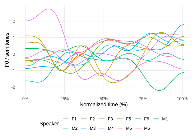
Most of the deviations are within 2 semitones relative to the median f0, but some (like those for speakers M5 and F6) can go beyond that threshold.
The last term, s(time_norm, token, bs = "fs", k = 5, m = 1), does something similar, but we limit the number of basis functions to five (k=5) in this case. Recall that token corresponds to repetitions of the same word and there should not be much variation between tokens. Note that the more basis functions we use, the more complex the model is and the longer it takes to compute.
Finally the argument discrete = TRUE is specific to the bam() method and helps to speed up the fitting of the model. The argument method = "fREML" instructs the program to use a (f)ast variant of the Restricted Maximum Likelihood (REML) in the fitting, specifically, the method to estimate the smoothing parameters. Using this particular combination (bam() with discrete = TRUE and fREML) is a practical way to minimize the time required for computing a model, especially a complex one.