10 Diagnosing models
The summary mainly tells us the estimates found by the model, it does not say much about whether the fitting of the model was adequate or not. We can achieve that by calling gam.check()
##
## Method: fREML   Optimizer: perf chol
## $grad
##  [1] -7.01e-05  5.83e-11  5.02e-12  2.69e-13 -1.04e-04 -7.43e-05  2.12e-10
##  [8] -1.59e-13  6.86e-11  1.99e-13 -4.52e-10
##
## $hess
##        [,1]      [,2]      [,3]      [,4]      [,5]      [,6]      [,7]
##    7.46e-05 -1.18e-04 -5.73e-05  8.18e-05  3.18e-07  1.93e-07  7.89e-04
##   -1.18e-04  2.60e+00  3.40e-02  3.26e-04  2.92e-05  2.47e-05  2.11e-01
##   -5.73e-05  3.40e-02  3.58e+00  1.07e-01 -6.66e-06 -4.24e-06 -4.37e-02
##    8.18e-05  3.26e-04  1.07e-01  3.30e+00 -8.82e-07  4.77e-07  1.72e-02
##    3.18e-07  2.92e-05 -6.66e-06 -8.82e-07  1.04e-04 -1.86e-08  1.58e-04
##    1.93e-07  2.47e-05 -4.24e-06  4.77e-07 -1.86e-08  7.43e-05 -7.47e-05
##    7.89e-04  2.11e-01 -4.37e-02  1.72e-02  1.58e-04 -7.47e-05  3.81e+01
##    4.53e-07 -9.64e-06  2.65e-05 -6.67e-06 -4.32e-08  6.06e-08 -5.83e-04
##    2.97e-04  8.60e-02  6.06e-03  1.27e-01  3.43e-05 -1.17e-05  1.75e+00
##   -5.54e-06  4.95e-07  4.60e-04 -2.68e-04 -5.54e-07 -7.20e-08  2.32e-04
## d -2.22e-03 -3.09e+00 -3.83e+00 -3.69e+00 -1.97e-04 -1.39e-04 -4.20e+01
##        [,8]      [,9]     [,10]     [,11]
##    4.53e-07  2.97e-04 -5.54e-06 -2.22e-03
##   -9.64e-06  8.60e-02  4.95e-07 -3.09e+00
##    2.65e-05  6.06e-03  4.60e-04 -3.83e+00
##   -6.67e-06  1.27e-01 -2.68e-04 -3.69e+00
##   -4.32e-08  3.43e-05 -5.54e-07 -1.97e-04
##    6.06e-08 -1.17e-05 -7.20e-08 -1.39e-04
##   -5.83e-04  1.75e+00  2.32e-04 -4.20e+01
##    1.60e+00 -4.20e-04  1.07e+00 -2.68e+00
##   -4.20e-04  3.78e+02  4.98e-02 -3.99e+02
##    1.07e+00  4.98e-02  1.01e+02 -1.04e+02
## d -2.68e+00 -3.99e+02 -1.04e+02  7.17e+03
##
## Model rank =  1268 / 1269
##
## Basis dimension (k) checking results. Low p-value (k-index<1) may
## indicate that k is too low, especially if edf is close to k'.
##
##                            k'      edf k-index p-value
## s(time_norm):Tone1   9.00e+00 1.00e+00    1.01    0.67
## s(time_norm):Tone2   9.00e+00 7.17e+00    1.01    0.64
## s(time_norm):Tone3   9.00e+00 8.66e+00    1.01    0.71
## s(time_norm):Tone4   9.00e+00 8.38e+00    1.01    0.63
## s(time_norm):GenderF 9.00e+00 1.00e+00    1.01    0.70
## s(time_norm):GenderM 9.00e+00 4.27e-04    1.01    0.67
## s(time_norm,Speaker) 1.10e+02 8.94e+01    1.01    0.68
## s(time_norm,token)   1.10e+03 1.01e+03    1.01    0.62
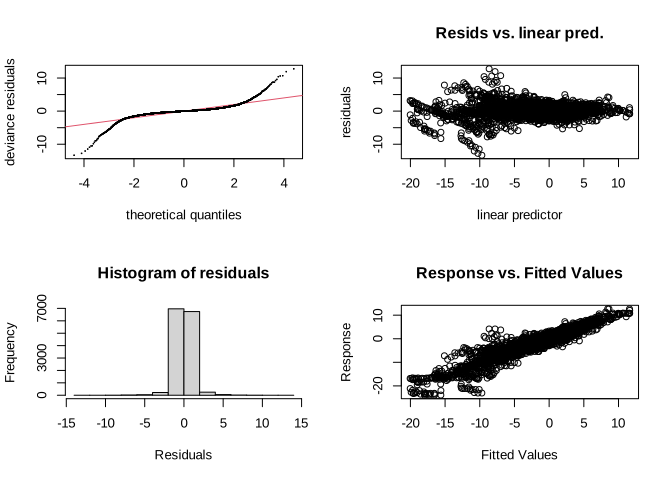
By default, this function returns a four-panel figure and some textual information.
10.1 Figures
To better understand these figures, it is useful to review the concept of “residuals.” For every data point (f0 in semitones, in our example), the model predicts a value based on the formula we have specified. A residual is the difference between the observed and the predicted values: \[ \mathrm{residual} = \mathrm{observed} - \mathrm{predicted} \]
A good model should have residuals that look random, i.e., without a visible pattern.
QQ-plot: In this plot, residuals should closely follow the diagonal red line. Look out for curves that deviate, particularly at the ends. Such deviations indicate that the residuals do not follow the distribution assumed by the model, which may be a sign of an imperfect fit.
Residual vs. linear predictor: A good fit will show a random cloud of points around zero, with no obvious patterns.
- Funnel shape: This indicates heteroscedasticity (meaning that the variance of the residuals changes depending on the predicted value)
- Curves or other patterns: These indicate that the model may be missing some structural relationship in the data.
Histogram of residuals: A good fit yields a bell-shaped and roughly symmetric histogram (without obvious skewness).
Response vs. fitted values: points scattered around a reference line, without systematic curvature.
In our case, we see some problems: the QQ-plot shows large deviations at both ends, and there are some patterns in the Residual vs. linear predictor plot. We will come back to this later.
10.2 Textual information
Because we used bam(), the output of gam.check() does not include information about full convergence (as it does when we use gam() instead). Instead, it shows
$grad: The gradient of the objective function (the function thatbam()is trying to minimize when fitting the model) which should be close to zero for all parameters. Large values can indicate that the model has not converged properly.$hess: The Hessian matrix (comprising the 2nd derivatives of the objective function) which is helpful to confirm whether the model has reached a minimum or not.
These two pieces of information are not usually reported. Instead, one should check that there is no convergence warning or error, and that the entries in $grad are all close to zero (this is the case in our example).
The bottom part of the textual output shows the basis dimensions. These parts are actually very important:
Model rank: It shows the number of independent dimensions in the model matrix. Ideally, we want a full rank, corresponding to a ratio of 1. If the ratio is much smaller than 1, it could indicate redundancy on the predictors, and it is worth investigating. In our case, we have a deficiency of 1 (1268/1269). This is usually not a problem.
k-indexvalues should generally be greater than or equal to 1, with non-significant p-values. A low k-index suggests the basis dimension k may be too small (the smooths are missing raises and dips that are genuinely present in the data). In that case, one should recompute the model increasing the numberkof the offending smooth.
The model-checking results indicate that the model has no obvious convergence problems and that the basis dimensions of the smooth terms are adequate. However, the residual diagnostics reveal some departures from the expected patterns. We will return to these issues later and consider how the model can be improved. In our case, we see some problems: the QQ-plot shows large deviations at both ends, and there are some patterns in the Residual vs. linear predictor plot. We will come back to this later.
10.3 Reproducibility
Running gam.check() several times will produce similar but not identical results. This is mainly because this function uses random numbers to generate the diagnostics.
This variation can be problematic when reporting the results in an article. One way to solve that is to set the seed of the random number generator, so that every time the code is run, it uses the same seed and therefore the results are identical. This can be achieved by
set.seed(54)
gam.check(model_02_noAR)
the 54 can be replaced by any entire number.