5 Frequency normalization

The overall f0 difference between male and female speakers is not that interesting. Besides, this large difference (sometimes spanning about one octave) hinders the discovery of other smaller differences in the trajectories.

We eliminate these biological differences by expressing f0 in semitones¹ relative to the median f0 of a given speaker. A semitone is the interval between a black key and the closest white key in a piano (in fact, between two adjacent keys), and it can be computed as

\[ F0_{\mathrm{st}} = 12 \times \log_2\left( \frac{F0}{F0_{\mathrm{median,speaker}}} \right) \]

This is achieved in R with

speaker_median <- tapply(f0_df$F0, f0_df$Speaker, median, na.rm = TRUE)
f0_df$F0_median_speaker <- speaker_median[f0_df$Speaker]
f0_df$F0_st <- 12 * log2(f0_df$F0 / f0_df$F0_median_speaker)

Note that we added na.rm = TRUE (i.e., ignore those “not available” entries) in the computation of the median. This is important because the f0 extraction algorithm fails sometimes, producing na values which will yield a na median too.

We can see the result of this transformation with

p <- ggplot(
  f0_df,
  aes(
    x = t_ms / 1000, y = F0_st,
    color = repetition, linetype = repetition,
    group = token
  )) +
  geom_line(alpha = 0.7, linewidth = 0.5) +
  facet_grid(
    rows = vars(Speaker), cols = vars(Tone),
    as.table = TRUE, switch = "y") +
  labs(
    title = NULL,
    x = "Time/s",
    y = "F0/semitones re. speaker median"
  ) +
  scale_y_continuous(n.breaks = 3) +
  guides(color = guide_legend(position = "bottom")) +
  theme_minimal(base_size = 18) +
  theme(
    axis.text.x = element_text(angle = 90, hjust = 1)
  )
p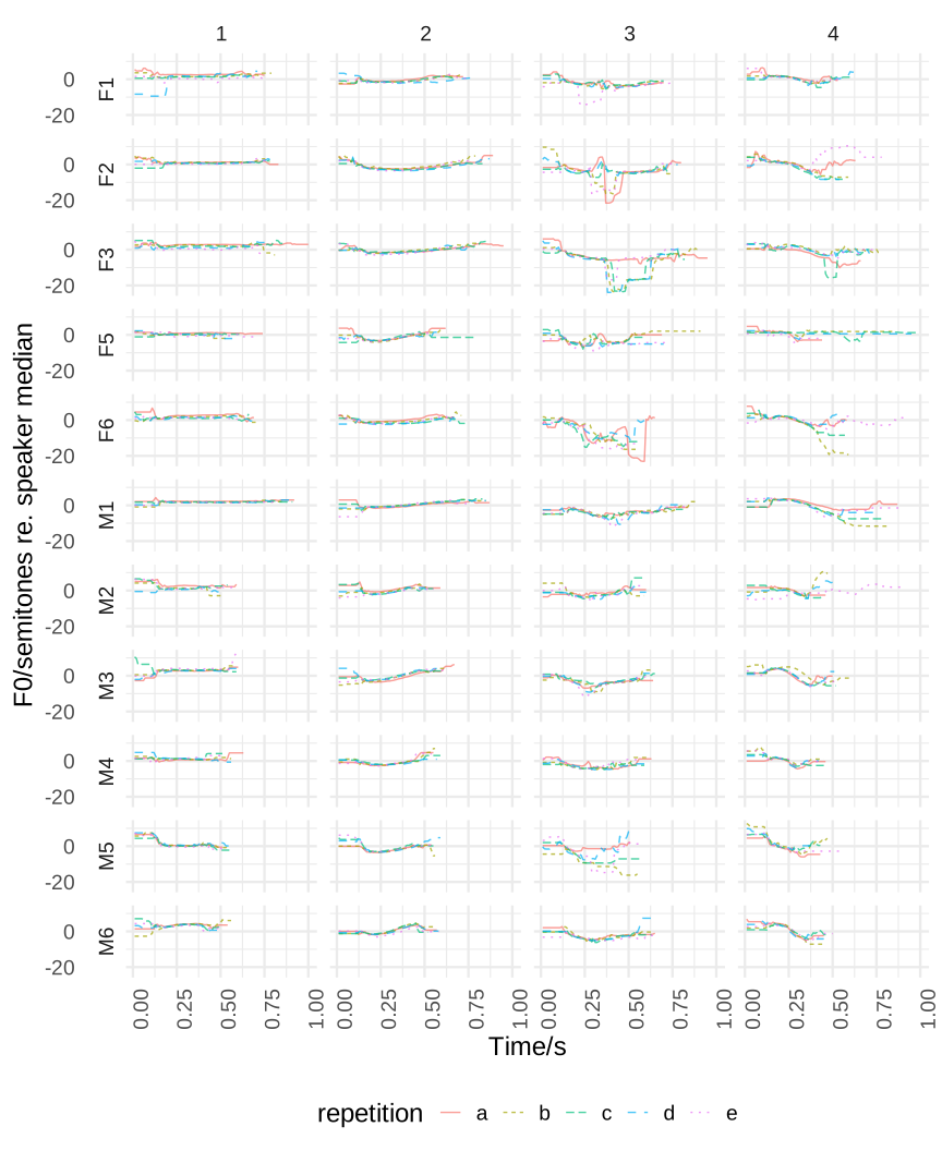

---

1. Sometimes cents are preferred over semitones. A cent is one hundredth of a semitone. In those cases, replace the 12 by 1200 in the formula above↩︎