13 Post-hoc analysis
In the previous chapter, we decided to use the model model_01_ac for our analysis. Our model answers the question “do the f0 trajectories vary by tone, once we have accounted for the fact that speakers may produce these tones differently, and that individual recordings may also differ from each other?”
It is convenient to rename it so if later on we decide to refine or change the model, we do not need to go through all the following instances of the code changing the name of the model.
Let us now summarize the model
##
## Family: gaussian
## Link function: identity
##
## Formula:
## F0_st ~ Tone + s(time_norm, by = Tone, k = 10, bs = "cr") + s(time_norm,
##     Speaker, bs = "fs", k = 10, m = 1) + s(time_norm, token,
##     bs = "fs", k = 5, m = 1)
##
## Parametric coefficients:
##             Estimate Std. Error t value Pr(>|t|)
## (Intercept)   1.6931     0.2499   6.775 1.30e-11 ***
## Tone2        -1.9665     0.2554  -7.699 1.47e-14 ***
## Tone3        -5.2041     0.2554 -20.378  < 2e-16 ***
## Tone4        -1.7303     0.2561  -6.756 1.47e-11 ***
## ---
## Signif. codes:  0 '***' 0.001 '**' 0.01 '*' 0.05 '.' 0.1 ' ' 1
##
## Approximate significance of smooth terms:
##                          edf   Ref.df      F p-value
## s(time_norm):Tone1     1.306    1.401  1.329   0.335
## s(time_norm):Tone2     6.395    7.356  6.870  <2e-16 ***
## s(time_norm):Tone3     8.285    8.746 25.786  <2e-16 ***
## s(time_norm):Tone4     8.078    8.637 13.934  <2e-16 ***
## s(time_norm,Speaker)  85.671  109.000  4.358  <2e-16 ***
## s(time_norm,token)   872.639 1096.000  8.570  <2e-16 ***
## ---
## Signif. codes:  0 '***' 0.001 '**' 0.01 '*' 0.05 '.' 0.1 ' ' 1
##
## R-sq.(adj) =  0.903   Deviance explained =   91%
## fREML =  16943  Scale est. = 1.1777    n = 14357
The summary shows the parametric coefficients on top (as we observed in Chapter 8), and the smooth terms below them. The parametric values only contain tone, and it is telling us that Tone 1 (the intercept) is on average 1.7 semitones higher than the speaker median, while Tone 2 is -0.27 semitones (or 1.96 semitones lower than Tone 1: \(1.685 - 1.956 = -0.27\)), and so on:
| Estimate | |
|---|---|
| Tone 1 | 1.685 |
| Tone 2 | −0.270 |
| Tone 3 | −3.511 |
| Tone 4 | −0.035 |
This table is telling us the differences in overall f0, but says nothing about the actual tone shapes. That information is in the smooth terms. Let us focus on the \(edf\) (effective degrees of freedom) and the \(p\)-value. \(Edf\) tells us about the curvature of the term, while the \(p\)-value from the \(F\)-statistic tells us whether the term, taken as a whole, reliably differs from a flat line at zero. For a low-edf term like Tone 1 below, these two together mean the curve is both non-curvy and indistinguishable from flat, but for higher edf terms, a non-significant \(p\)-value does not guarantee the curve is constant everywhere, it is worth plotting to check.
Tone 1: for this tone \(edf\) = 1.1 and \(p = .161\). I.e., the curve is close to a straight line (as per the \(edf\)) and it is constant throughout the whole period (as per the \(p\)-value). Note that straight line increasing/decreasing throughout the whole period would have a similar \(edf\), but not necessarily the same \(p\)-value. Tone 1 (55) is a high leveled tone, and this is confirmed here: the parametric coefficients tell us that this is the tone with the highest average f0, and the smooth terms tells us that is flat.
Other tones: the remaining tones have larger \(edf\) (from the \(k'=9\)—see its
gam.check()in last chapter—, these smooths are using between 6 and 9), indicating that the tones have dips and rises, and all \(p\)-values are \(<.05\).Random smooths: Both are significant, implying that, as we expected, there is variability between speakers and between repetitions.
Deviance explained: The summary shows a good fit (91%), i.e., the variance in the data is explained by the model as a whole ()tone identity and its time trajectory), together with speaker and token variability.
To better discuss these results is always a good idea to plot the model predictions:
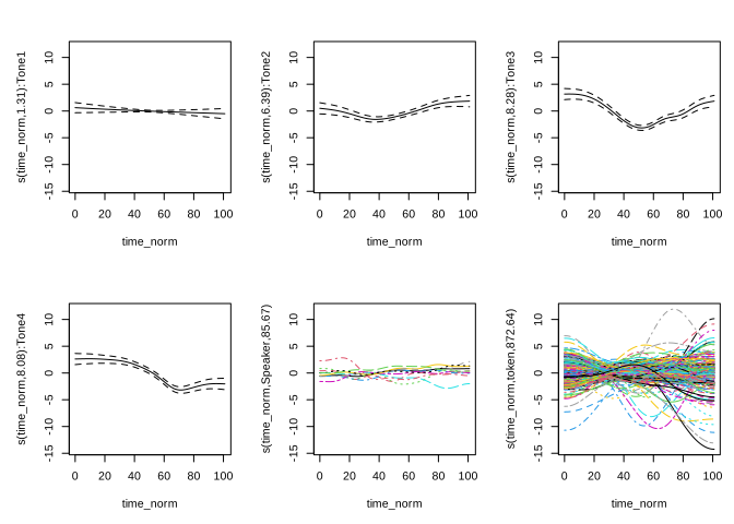
This figure shows the f0 trajectories for each tone, along with the random effects in a single page. The seWithMean argument changes the confidence interval by also including that of the intercept. This is a more conservative way to see if the traces are different from 0. Note also that this figure only shows the shape of the tones and not their relative height.
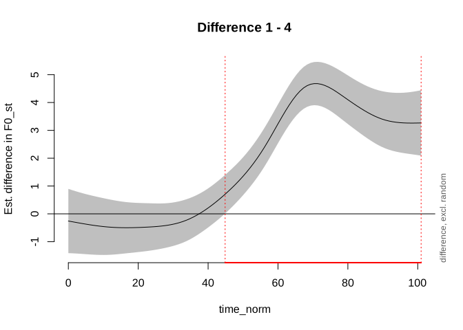
Just by looking at these individual plots, we could tell that some tones are different from each other. But, we would like to have a numeric way to assess where these trajectories are different. For example, Tone 1 and 4 both start somewhat high, where do they start being different? We could answer that with the plot_diff() function
## Summary:
## * time_norm : numeric predictor; with 100 values ranging from 0.000000 to
100.961538.
## * Speaker : factor; set to the value(s): M1. (Might be canceled as random
effect, check below.)
## * token : factor; set to the value(s): F3_1_a. (Might be canceled as random
effect, check below.)
## * NOTE : The following random effects columns are canceled:
s(time_norm,Speaker),s(time_norm,token)
##
##
## time_norm window(s) of significant difference(s):
##  44.871795 - 100.961538
This plot excludes random smooth terms, so the results shown are not for a particular speaker or repetition (token) but for the population, as predicted by the model. Note that the summary of the plot is somewhat confusing: it first says that Speaker is set to M1 and token to F3_1_a, but in the NOTE it says that random effects are canceled. The assignment of Speaker and token is only temporary, so believe the note in this case.
The plot also shows that during about the first \(45\%\) of the production, there is no significant difference between the two tones, but, from that point, Tone 1 is significantly higher than Tone 4, reaching up to about 4 semitones.
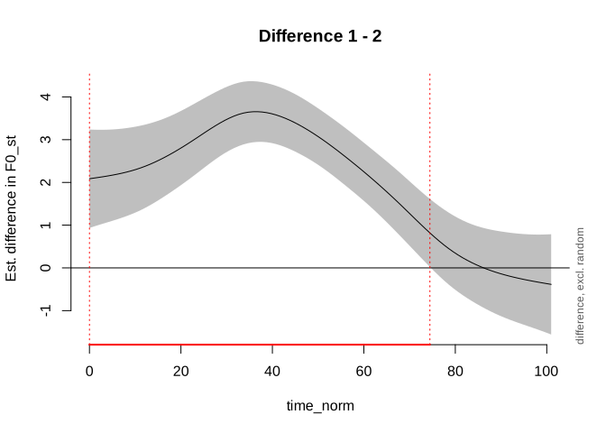
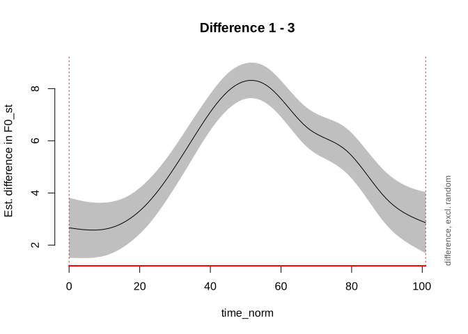
For completeness, here there are the remaining two-curve comparisons:
## Summary:
## * time_norm : numeric predictor; with 100 values ranging from 0.000000 to
100.961538.
## * Speaker : factor; set to the value(s): M1. (Might be canceled as random
effect, check below.)
## * token : factor; set to the value(s): F3_1_a. (Might be canceled as random
effect, check below.)
## * NOTE : The following random effects columns are canceled:
s(time_norm,Speaker),s(time_norm,token)
##
##
## time_norm window(s) of significant difference(s):
## 0.000000 - 74.446387## Summary:
## * time_norm : numeric predictor; with 100 values ranging from 0.000000 to
100.961538.
## * Speaker : factor; set to the value(s): M1. (Might be canceled as random
effect, check below.)
## * token : factor; set to the value(s): F3_1_a. (Might be canceled as random
effect, check below.)
## * NOTE : The following random effects columns are canceled:
s(time_norm,Speaker),s(time_norm,token)
##
##
## time_norm window(s) of significant difference(s):
## 0.000000 - 100.961538## Summary:
## * time_norm : numeric predictor; with 100 values ranging from 0.000000 to
100.961538.
## * Speaker : factor; set to the value(s): M1. (Might be canceled as random
effect, check below.)
## * token : factor; set to the value(s): F3_1_a. (Might be canceled as random
effect, check below.)
## * NOTE : The following random effects columns are canceled:
s(time_norm,Speaker),s(time_norm,token)
##
##
## time_norm window(s) of significant difference(s):
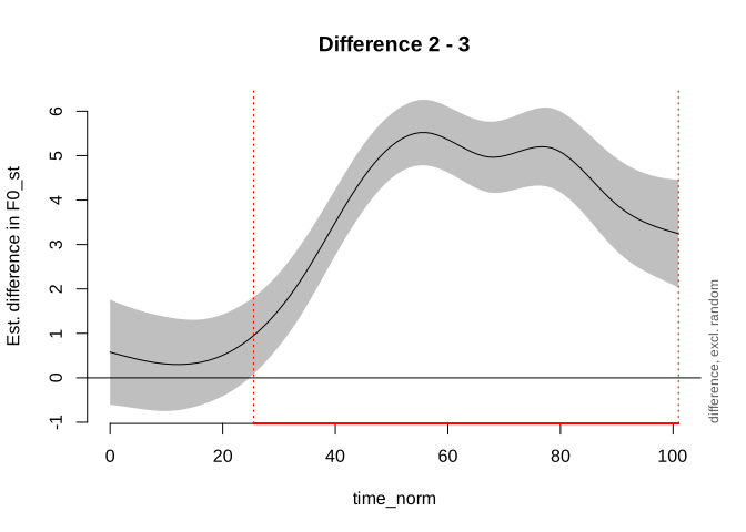
## 25.495338 - 100.961538## Summary:
## * time_norm : numeric predictor; with 100 values ranging from 0.000000 to
100.961538.
## * Speaker : factor; set to the value(s): M1. (Might be canceled as random
effect, check below.)
## * token : factor; set to the value(s): F3_1_a. (Might be canceled as random
effect, check below.)
## * NOTE : The following random effects columns are canceled:
s(time_norm,Speaker),s(time_norm,token)
##
##
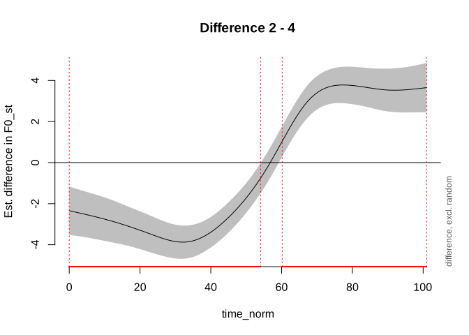
## time_norm window(s) of significant difference(s):
##  0.000000 - 54.050117
## 60.168998 - 100.961538## Summary:
## * time_norm : numeric predictor; with 100 values ranging from 0.000000 to
100.961538.
## * Speaker : factor; set to the value(s): M1. (Might be canceled as random
effect, check below.)
## * token : factor; set to the value(s): F3_1_a. (Might be canceled as random
effect, check below.)
## * NOTE : The following random effects columns are canceled:
s(time_norm,Speaker),s(time_norm,token)
##
##
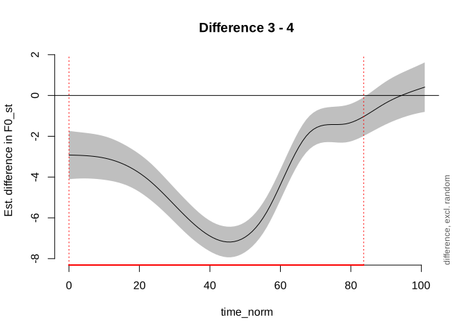
## time_norm window(s) of significant difference(s):
##  0.000000 - 83.624709
plot_diff() is a correct way to assess the difference between different smooths. It separates periods of significant difference from those periods where the curves are essentially indistinguishable from each other. This difference also includes the parametric coefficients, unlike the shape-only plots shown earlier.
13.1 Population-level curves
It is sometimes convenient to plot the predicted trajectories in a single plot, for reporting, for example. This could be achieved by predicting the traces from the model.
pred_grid <- expand.grid(
  time_norm = seq(0, 100, length.out = 100),
  Tone      = levels(f0_df$Tone)
)

pred_grid$Speaker <- f0_df$Speaker[1]   # placeholder, excluded below
pred_grid$token   <- f0_df$token[1]     # placeholder, excluded below

pred <- predict(
  gam_model,
  newdata = pred_grid,
  exclude = c("s(time_norm,Speaker)", "s(time_norm,token)"),
  se.fit  = TRUE
)

pred_grid$fit <- pred$fit
pred_grid$se  <- pred$se.fit
pred_grid$lower <- pred_grid$fit - 1.96 * pred_grid$se
pred_grid$upper <- pred_grid$fit + 1.96 * pred_grid$se

p_gam <- ggplot(pred_grid, aes(x = time_norm, y = fit, color = Tone, fill = Tone)) +
  geom_ribbon(aes(ymin = lower, ymax = upper), alpha = 0.2, color = NA) +
  geom_line(linewidth = 1) +
  labs(x = "Normalized time/%", y = "f0/semitones") +
  theme_minimal(14)

p_gam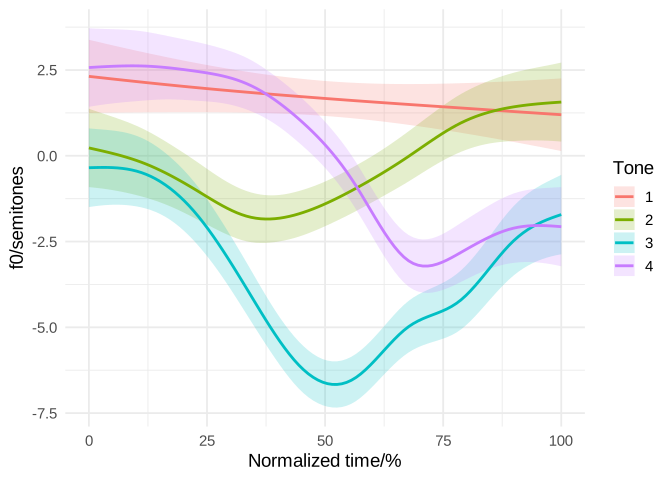
The plot includes the predicted traces along with the 95% confidence interval around them. Disjoint CIs are strong evidence of significant difference. Overlapping CIs, on the other hand, do not always indicate non-significance. This plot could be added to illustrate the differences between Mandarin tones in a report, while the numeric differences should be drawn from the plot_diff() and the summary() of the model.