12 Comparing models
We first created a model without taking into account the autocorrelation in the residuals (model_02_noAR) and in the previous chapter we included such an effect in model_02_ac. When we have several models, we would like to compare them in order to select the best one. We can do that with
## model_02_noAR: F0_st ~ Tone + Gender + s(time_norm, by = Tone, k = 10, bs = "cr") +
##     s(time_norm, by = Gender, k = 10, bs = "cr") + s(time_norm,
##     Speaker, bs = "fs", k = 10, m = 1) + s(time_norm, token,
##     bs = "fs", k = 5, m = 1)
##
## model_02_ac: F0_st ~ Tone + Gender + s(time_norm, by = Tone, k = 10, bs = "cr") +
##     s(time_norm, by = Gender, k = 10, bs = "cr") + s(time_norm,
##     Speaker, bs = "fs", k = 10, m = 1) + s(time_norm, token,
##     bs = "fs", k = 5, m = 1)
##
## Model model_02_ac preferred: lower fREML score (7082.871), and equal df (0.000).
## -----
##           Model    Score Edf Difference    Df
## 1 model_02_noAR 24023.34  10
## 2   model_02_ac 16940.47  10  -7082.871 0.000
##
## AIC difference: 12403.22, model model_02_ac has lower AIC.
This function first output the two models being compared and then suggests which model should be preferred and why. In our case, the model including the autocorrelation is preferred because it has a lower fREML score, lower Akaike’s Information Criterion (AIC) and equal degrees of freedom.
The same function could be used to test whether a term of the model’s formula (a factor, interaction, etc.) increases the fit of the model.
To illustrate that, let us first create a model without the effect of Gender by removing both the parameter and the smooth:
model_01_ac <- bam(F0_st ~
    Tone +
    s(time_norm, by = Tone, k = 10, bs = "cr") +
    s(time_norm, Speaker, bs = "fs", k = 10, m = 1) +
    s(time_norm, token, bs = "fs", k = 5, m = 1),
    data = f0_df,
    method = "fREML",
    discrete = TRUE,
    AR.start = f0_df$start_event,
    rho = rho_est
)
## Warning in gam.side(sm, X, tol = .Machine$double.eps^0.5): model has repeated
## 1-d smooths of same variable.- Note that this model uses the same autocorrelation estimate (\(\rho\)) as before. This matters: re-estimating \(\rho\) separately for each model would let the AR correction itself vary across models, confounding any comparison between them. So we estimate \(\rho\) once, from the most complex model we consider, and reuse that fixed value in all simpler models, as we have done here.
Now we can compare the two models which differ on the presence/absence of Gender as a factor.
## model_01_ac: F0_st ~ Tone + s(time_norm, by = Tone, k = 10, bs = "cr") + s(time_norm,
##     Speaker, bs = "fs", k = 10, m = 1) + s(time_norm, token,
##     bs = "fs", k = 5, m = 1)
##
## model_02_ac: F0_st ~ Tone + Gender + s(time_norm, by = Tone, k = 10, bs = "cr") +
##     s(time_norm, by = Gender, k = 10, bs = "cr") + s(time_norm,
##     Speaker, bs = "fs", k = 10, m = 1) + s(time_norm, token,
##     bs = "fs", k = 5, m = 1)
##
## Chi-square test of fREML scores
## -----
##         Model    Score Edf Difference    Df p.value Sig.
## 1 model_01_ac 16943.47   8
## 2 model_02_ac 16940.47  10      2.996 2.000   0.050  *
## Warning in compareML(model_01_ac, model_02_ac): Only small difference in fREML...## AIC difference: -0.24, model model_01_ac has lower AIC.As before, we have the two models on top, and their comparison at the bottom. Here we have an interesting contradiction: The Chi-square test of fREML scores suggests that we should accept model_02_ac since it has a small but significant difference in fREML relative to model_01_ac (using the common 5% criterion for significance). However, the AIC suggests that we should accept model_01_ac since its AIC is lower than that of model_02_ac. Note that the AIC difference is only -0.17. At this level, the two models are basically indistinguishable.
Let us plot the data once more, this time grouping by Gender and Tone:
p = ggplot(f0_df, aes(
  x = t_ms,
  y = F0_st,
  color = Gender,
  linetype = repetition,
  group = token
)) +
  geom_line(alpha = 0.7, linewidth = 0.3) +
  facet_wrap(vars(Tone), nrow = 4, as.table = TRUE) +
  labs(
    title = NULL,
    x = "Time/ms",
    y = "F0/semitones re. speaker median"
  ) +
  theme_minimal(base_size = 14)

p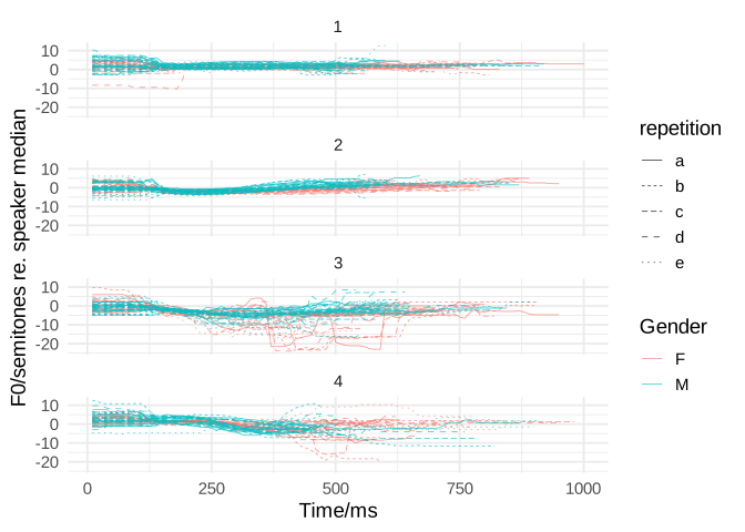
This plot is very revealing: Whereas the pitch production is rather static (it changes little over time), some of the traces have abrupt changes between consecutive samples. These abrupt changes are unnatural and are probably artifacts of the pitch tracking algorithm.
Let us check where are these large f0 jumps located:
f0_df <- f0_df %>%
  arrange(token, t_ms) %>%
  group_by(token) %>%
  mutate(F0_st_diff = F0_st - lag(F0_st)) %>%
  ungroup()

print(n = 100,
  f0_df %>%
    mutate(likely_error = abs(F0_st_diff) > 6) %>%
    filter(likely_error) %>%
    select(
      Speaker, Tone, Gender, token,
      F0_st, time_norm, F0_st_diff, likely_error
    )
)
## # A tibble: 24 × 8
## Speaker Tone Gender token F0_st time_norm F0_st_diff likely_error
## <fct> <fct> <fct> <fct> <dbl[1d]> <dbl> <dbl[1d]> <lgl[1d]>
## 1 F1 1 F F1_1_d 1.29 27.0 7.97 TRUE
## 2 F1 3 F F1_3_e -13.0 28.8 -10.1 TRUE
## 3 F2 3 F F2_3_a -21.6 45.5 -22.6 TRUE
## 4 F2 3 F F2_3_a -3.97 58.1 6.91 TRUE
## 5 F2 3 F F2_3_b -4.19 56.5 8.26 TRUE
## 6 F2 3 F F2_3_c 0.540 47.8 6.51 TRUE
## 7 F2 3 F F2_3_e -16.7 38.0 -16.7 TRUE
## 8 F2 3 F F2_3_e -8.58 57.1 6.63 TRUE
## 9 F3 3 F F3_3_b -17.1 42.8 -9.86 TRUE
## 10 F3 3 F F3_3_b -10.1 70.9 6.17 TRUE
## 11 F3 3 F F3_3_c -23.2 50.7 -10.5 TRUE
## 12 F3 3 F F3_3_c -7.42 73.0 8.93 TRUE
## 13 F3 3 F F3_3_d -23.9 47.7 -15.1 TRUE
## 14 F3 3 F F3_3_d -4.99 79.9 11.2 TRUE
## 15 F3 3 F F3_3_e -12.2 47.4 -6.47 TRUE
## 16 F3 3 F F3_3_e -7.03 56.6 10.2 TRUE
## 17 F3 4 F F3_4_c -13.4 64.7 -10.2 TRUE
## 18 F3 4 F F3_4_c -2.25 74.7 13.2 TRUE
## 19 F6 3 F F6_3_a -19.2 76.6 -13.0 TRUE
## 20 F6 3 F F6_3_a 0.394 92.2 23.4 TRUE
## 21 F6 3 F F6_3_d -0.521 87.2 11.0 TRUE
## 22 M5 3 M M5_3_d 5.50 83.3 8.92 TRUE
## 23 M5 3 M M5_3_e -14.5 48.6 -8.02 TRUE
## 24 M5 3 M M5_3_e -2.75 71.2 11.7 TRUEThe resulting list comprises instances where f0 jumped more than 6 semitones in 10 ms. This is unexpected for typical speakers, so we should be suspicious of these data. Most of these changes appear in Tone 3 (213) which is often glottalized. Glottalization poses a major difficulty for many f0 trackers.
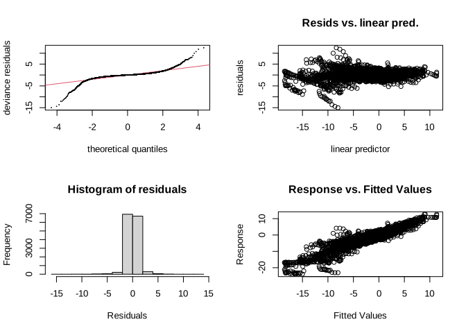
In this case, we will reject the model including the effect of Gender (model_02_ac) and accept the one with only the effect of Tone (model_01_ac). In a real case, we should check the f0 extraction before the statistical modeling, ensuring that the traces do not contain abrupt jumps. For this tutorial, we will use the current data, but just to illustrate the influence of the abnormal data on the model, here we fit a new model to the data with Tone 3 excluded, but first let us check model_01_ac
##
## Method: fREML   Optimizer: perf chol
## $grad
## [1] -2.56e-07  6.48e-08  9.90e-09 -1.38e-08 -9.95e-08 -1.06e-09 -4.11e-09
## [8]  3.99e-09  4.68e-07
##
## $hess
##        [,1]     [,2]      [,3]      [,4]      [,5]      [,6]      [,7]
##    0.025414 -0.02125 -0.006136  4.10e-03   0.06127  3.82e-04  1.70e-02
##   -0.021246  2.25024  0.007133 -1.72e-02   0.22178 -2.70e-04  7.80e-02
##   -0.006136  0.00713  3.222316  1.13e-01  -0.02431 -1.51e-04  3.02e-02
##    0.004105 -0.01716  0.112980  3.05e+00  -0.05849 -4.35e-05  8.45e-02
##    0.061272  0.22178 -0.024312 -5.85e-02  31.76387 -1.22e-02  2.01e+00
##    0.000382 -0.00027 -0.000151 -4.35e-05  -0.01220  3.08e+00  2.01e-03
##    0.017015  0.07805  0.030250  8.45e-02   2.01442  2.01e-03  2.73e+02
##   -0.001484  0.00171  0.000614  3.77e-05  -0.00434  7.62e-01  1.03e+00
## d -0.153240 -2.69747 -3.642282 -3.54e+00 -38.91071 -3.92e+00 -3.39e+02
##        [,8]     [,9]
##   -1.48e-03   -0.153
##    1.71e-03   -2.697
##    6.14e-04   -3.642
##    3.77e-05   -3.539
##   -4.34e-03  -38.911
##    7.62e-01   -3.925
##    1.03e+00 -339.376
##    8.97e+01  -96.944
## d -9.69e+01 7174.500
##
## Model rank =  1250 / 1250
##
## Basis dimension (k) checking results. Low p-value (k-index<1) may
## indicate that k is too low, especially if edf is close to k'.
##
##                           k'     edf k-index p-value
## s(time_norm):Tone1      9.00    1.31    0.97   0.020 *
## s(time_norm):Tone2      9.00    6.39    0.97   0.025 *
## s(time_norm):Tone3      9.00    8.28    0.97   0.030 *
## s(time_norm):Tone4      9.00    8.08    0.97   0.025 *
## s(time_norm,Speaker)  110.00   85.67    0.97   0.040 *
## s(time_norm,token)   1100.00  872.64    0.97   0.025 *
## ---
## Signif. codes:  0 '***' 0.001 '**' 0.01 '*' 0.05 '.' 0.1 ' ' 1
f0_df_no3 <- f0_df %>%
filter(Tone != "3") %>%
droplevels()
gam_model_no3 <- bam(F0_st ~
Tone +
s(time_norm, by = Tone, k = 10, bs = "cr") +
s(time_norm, Speaker, bs = "fs", k = 10, m = 1) +
s(time_norm, token, bs = "fs", k = 5, m = 1),
data = f0_df_no3,
method = "fREML",
discrete = TRUE,
AR.start = f0_df_no3$start_event,
rho = rho_est
)
summary(gam_model_no3)##
## Family: gaussian
## Link function: identity
##
## Formula:
## F0_st ~ Tone + s(time_norm, by = Tone, k = 10, bs = "cr") + s(time_norm,
## Speaker, bs = "fs", k = 10, m = 1) + s(time_norm, token,
## bs = "fs", k = 5, m = 1)
##
## Parametric coefficients:
## Estimate Std. Error t value Pr(>|t|)
## (Intercept) 1.687 0.176 9.58 <2e-16 ***
## Tone2 -1.963 0.207 -9.47 <2e-16 ***
## Tone4 -1.726 0.208 -8.31 <2e-16 ***
## ---
## Signif. codes: 0 '***' 0.001 '**' 0.01 '*' 0.05 '.' 0.1 ' ' 1
##
## Approximate significance of smooth terms:
## edf Ref.df F p-value
## s(time_norm):Tone1 2.13 2.39 0.89 0.31
## s(time_norm):Tone2 7.15 7.96 9.52 <2e-16 ***
## s(time_norm):Tone4 8.43 8.78 20.21 <2e-16 ***
## s(time_norm,Speaker) 82.73 109.00 3.97 <2e-16 ***
## s(time_norm,token) 684.71 822.00 13.43 <2e-16 ***
## ---
## Signif. codes: 0 '***' 0.001 '**' 0.01 '*' 0.05 '.' 0.1 ' ' 1
##
## R-sq.(adj) = 0.927 Deviance explained = 93.2%
## fREML = 8867.2 Scale est. = 0.57106 n = 10630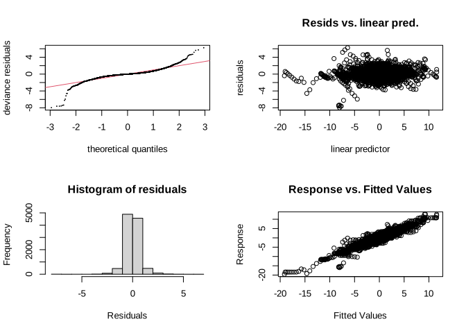
##
## Method: fREML   Optimizer: perf chol
## $grad
## [1] -5.35e-08  1.34e-09 -1.47e-09  1.75e-08 -2.98e-09  1.19e-08  4.32e-09
## [8]  4.05e-09
##
## $hess
##        [,1]     [,2]      [,3]      [,4]      [,5]      [,6]      [,7]     [,8]
##    0.330350 -0.03810  2.10e-02   0.03668  9.56e-04  1.13e-02 -1.79e-03   -0.563
##   -0.038104  2.76785  2.26e-03   0.25915 -1.60e-04  9.19e-02  8.10e-04   -3.076
##    0.021027  0.00226  3.37e+00   0.01582 -4.68e-05  6.96e-02 -2.43e-04   -3.715
##    0.036683  0.25915  1.58e-02  30.61318 -1.73e-03  4.01e+00 -3.21e-03  -38.507
##    0.000956 -0.00016 -4.68e-05  -0.00173  1.63e+00  1.26e-03  1.14e+00   -2.858
##    0.011263  0.09188  6.96e-02   4.00864  1.26e-03  2.29e+02  7.82e-01 -268.232
##   -0.001795  0.00081 -2.43e-04  -0.00321  1.14e+00  7.82e-01  6.93e+01  -74.123
## d -0.562608 -3.07560 -3.71e+00 -38.50710 -2.86e+00 -2.68e+02 -7.41e+01 5312.000
##
## Model rank =  965 / 965
##
## Basis dimension (k) checking results. Low p-value (k-index<1) may
## indicate that k is too low, especially if edf is close to k'.
##
##                          k'    edf k-index p-value
## s(time_norm):Tone1     9.00   2.13    0.99    0.17
## s(time_norm):Tone2     9.00   7.15    0.99    0.15
## s(time_norm):Tone4     9.00   8.43    0.99    0.21
## s(time_norm,Speaker) 110.00  82.73    0.99    0.18
## s(time_norm,token)   825.00 684.71    0.99    0.18
The diagnostics of the latter model are better behaved than in the model_01_ac model which includes Tone 3 (the tone with most abnormal f0 jumps).