11 Introducing autocorrelation correction

The f0 measurements are taken every 10 ms within the same token. Residuals from consecutive time points in the same trajectory are almost certainly correlated. If a model underpredicts f0 at a given time, it is very likely to still be underpredicting at short lags after that point in time because f0 does not jump abruptly between consecutive samples.

Let us estimate the autocorrelation in the residuals of our model within tokens:

acf(resid(model_02_noAR), main = "ACF of residuals")

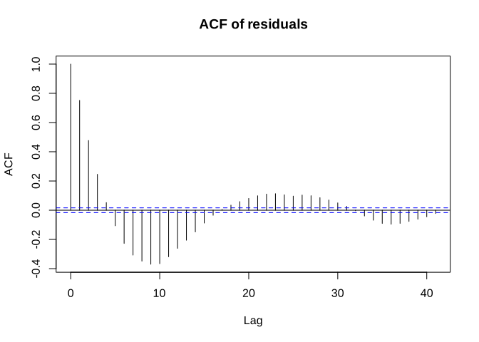
The figure above shows the autocorrelation at different lags. At no lag, the autocorrelation is 1 (as expected), to account for the autocorrelation in each token, we want the autocorrelation of two consecutive samples

rho_est <- acf(resid(model_02_noAR), lag.max = 1, plot = FALSE)$acf[2]
rho_est

## [1] 0.7515731

This value can be used in our model as

model_02_ac <- bam(F0_st ~
    Tone + Gender +
    s(time_norm, by = Tone, k = 10, bs = "cr") +
    s(time_norm, by = Gender, k = 10, bs = "cr") +
    s(time_norm, Speaker, bs = "fs", k = 10, m = 1) +
    s(time_norm, token, bs = "fs", k = 5, m = 1),
    data = f0_df,
    method = "fREML",
    discrete = TRUE,
    AR.start = f0_df$start_event,
    rho = rho_est
)

## Warning in gam.side(sm, X, tol = .Machine$double.eps^0.5): model has repeated
## 1-d smooths of same variable.

The last two lines indicate where the first sample is located for each token, and the aforementioned 1-lag autocorrelation.